milRex

Getting Data

Querying the Military Expenditure Database by SIPRI can be done through their website, however, the resulting xlsx is rather tedious to parse because of some formatting choices taken by the team.

Hence this function makes it easy to directly import this database to R and parse not only the different indicators, but also the associated footnotes.

The following code is all you need to query data from their website.

library(milRex)
milex <- sipri_get_data(indicator = "constantUSD")

The available indicators are:

Description	indicator
Constant (2022) US$	constantUSD
Current US$	currentUSD
Share of GDP	shareOfGDP
Share of Govt. spending	shareGovt
Regional totals	regionalTotals
Local currency financial years	currencyFY
Local currency calendar years	currencyCY
Per capita	perCapita
all of the above	all

Aggregating data by regions

The package also comes with a pre-packaged data-frame that allows you to merge SIPRIs regional coding to the data-frame.

We join the two dataframes by the country names, exclude values for 1991 where a total cannot be calculated because the Soviet Union is missing in the data and then sum the values acorss regions and years.

library(dplyr)
library(lubridate)

milex_regional <- milex |> 
  dplyr::left_join(milRex::sipri_regions) |>  ## join data
  dplyr::summarise(value = sum(value, na.rm = T), 
                   .by = c(region, year)) |> ## sum up 
  dplyr::filter(year >= 1988)|> ## exclude values pre-1988
  dplyr::mutate(value = if_else(year == 1991, 0, value)) |> # exclude 1991
  dplyr::mutate(year = paste(year, "01-01") |> 
                  lubridate::ymd()) # format dates nicely 

Plotting the data

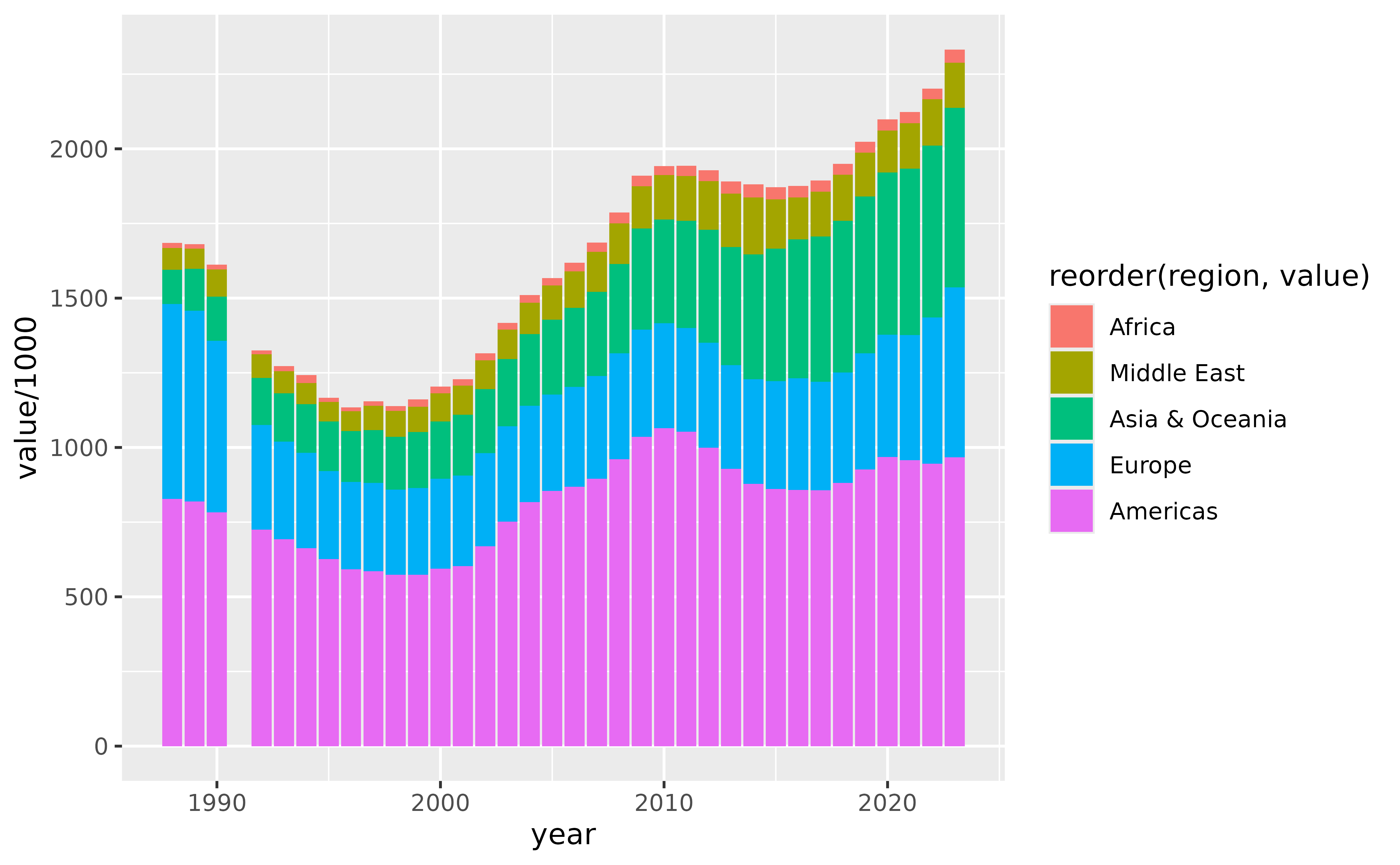
Now we can replicate a common graph used by SIPRI to show military spending by regions.

library(ggplot2)

ggplot2::ggplot(milex_regional) +
  ggplot2::geom_col(ggplot2::aes(year, value/1000, 
                                 fill = reorder(region, value)))

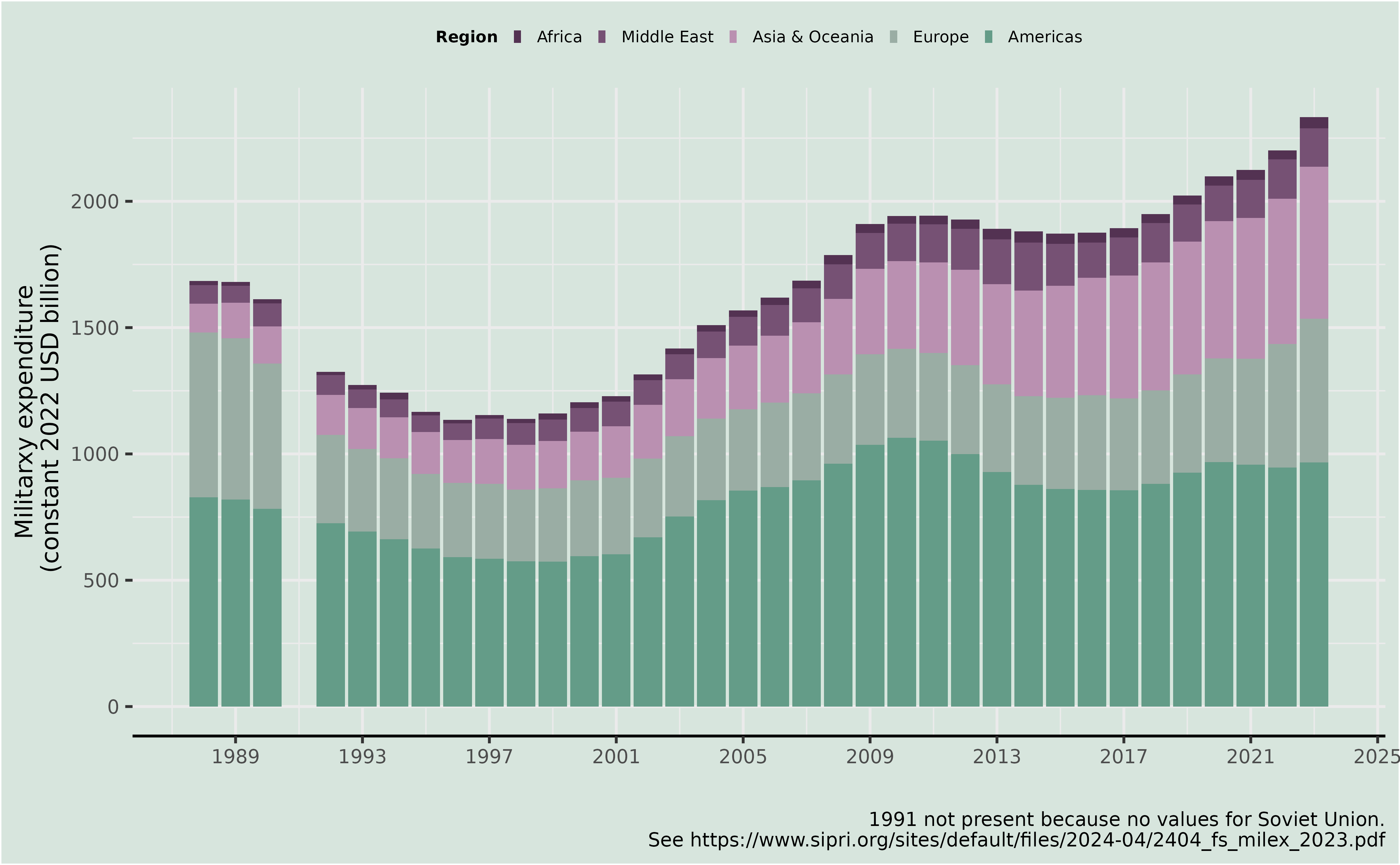
This looks rather ugly, but we can approximate the styling of SIPRI, as in the plot here:

ggplot(milex_regional) +
  geom_col(aes(year, value/1000, fill = reorder(region, value))) +
  labs(y = "Militarxy expenditure\n (constant 2022 USD billion)",
       caption = "1991 not present because no values for Soviet Union.\n See https://www.sipri.org/sites/default/files/2024-04/2404_fs_milex_2023.pdf", 
       fill = "Region",
       x = "") + 
  theme_bw() +
  theme(plot.background = element_rect(fill = rgb(215, 229, 221, 
                                                  maxColorValue = 255)),
        panel.background = element_rect(fill = rgb(215, 229, 221, 
                                                  maxColorValue = 255)),
        legend.background = element_rect(fill = rgb(215, 229, 221, 
                                                  maxColorValue = 255)),
        legend.position = "top",
        legend.text = element_text(size = 6),
        legend.title = element_text(size = 6,face  = "bold"),
        panel.border = element_blank(),
        axis.line.x = element_line(),
        text = element_text(size = 9),
        legend.key.size = unit(0.05, 'in'))+
  scale_fill_manual(values = 
                      c(
                        rgb(83,50,82, maxColorValue = 255),
                        rgb(118,81,116, maxColorValue = 255),
                        rgb(186,144,177, maxColorValue = 255),
                        rgb(154,173,164, maxColorValue = 255),
                        rgb(100,156,136, maxColorValue = 255)
                      ))+
  scale_x_date(breaks = "4 years",date_labels = "%Y")